pacman::p_load(tidytext, widyr, wordcloud, DT, ggwordcloud, textplot, lubridate, hms,
tidyverse, tidygraph, ggraph, igraph)Hands-on Ex5
Visualising and Analysing Text Data with R: tidytext methods
Getting Started
Loading Required R Package Libraries
The code chunk below loads the following libraries:
- tidytext,
- tidyverse (mainly readr, purrr, stringr, ggplot2)
- widyr, - wordcloud and ggwordcloud,
- textplot (required igraph, tidygraph and ggraph, )
- DT,
- lubridate and hms.
Importing Multiple Text Files from Multiple Folders
Creating a folder list
news20 <- "data/20news/"Define a function to read all files from a folder into a data frame
read_folder <- function(infolder) {
  tibble(file = dir(infolder,
                    full.names = TRUE)) %>%
    mutate(text = map(file,
                      read_lines)) %>%
    transmute(id = basename(file),
              text) %>%
    unnest(text)
}
Reading in all the messages from the 20news folder
raw_text <- tibble(folder =
                     dir(news20,
                         full.names = TRUE)) %>%
  mutate(folder_out = map(folder,
                          read_folder)) %>%
  unnest(cols = c(folder_out)) %>%
  transmute(newsgroup = basename(folder),
            id, text)
write_rds(raw_text, "data/rds/news20.rds")
Things to learn from the code chunk above:
- read_lines() of readr package is used to read up to n_max lines from a file.
- map() of purrr package is used to transform their input by applying a function to each element of a list and returning an object of the same length as the input.
- unnest() of dplyr package is used to flatten a list-column of data frames back out into regular columns.
- mutate() of dplyr is used to add new variables and preserves existing ones;
- transmute() of dplyr is used to add new variables and drops existing ones.
- read_rds() is used to save the extracted and combined data frame as rds file for future use.
Initial EDA
The code chunk below gives the Figure that shows the frequency of messages by newsgroup.
raw_text %>%
  group_by(newsgroup) %>%
  summarize(messages = n_distinct(id)) %>%
  ggplot(aes(messages, newsgroup)) +
  geom_col(fill = "lightblue") +
  labs(y = NULL)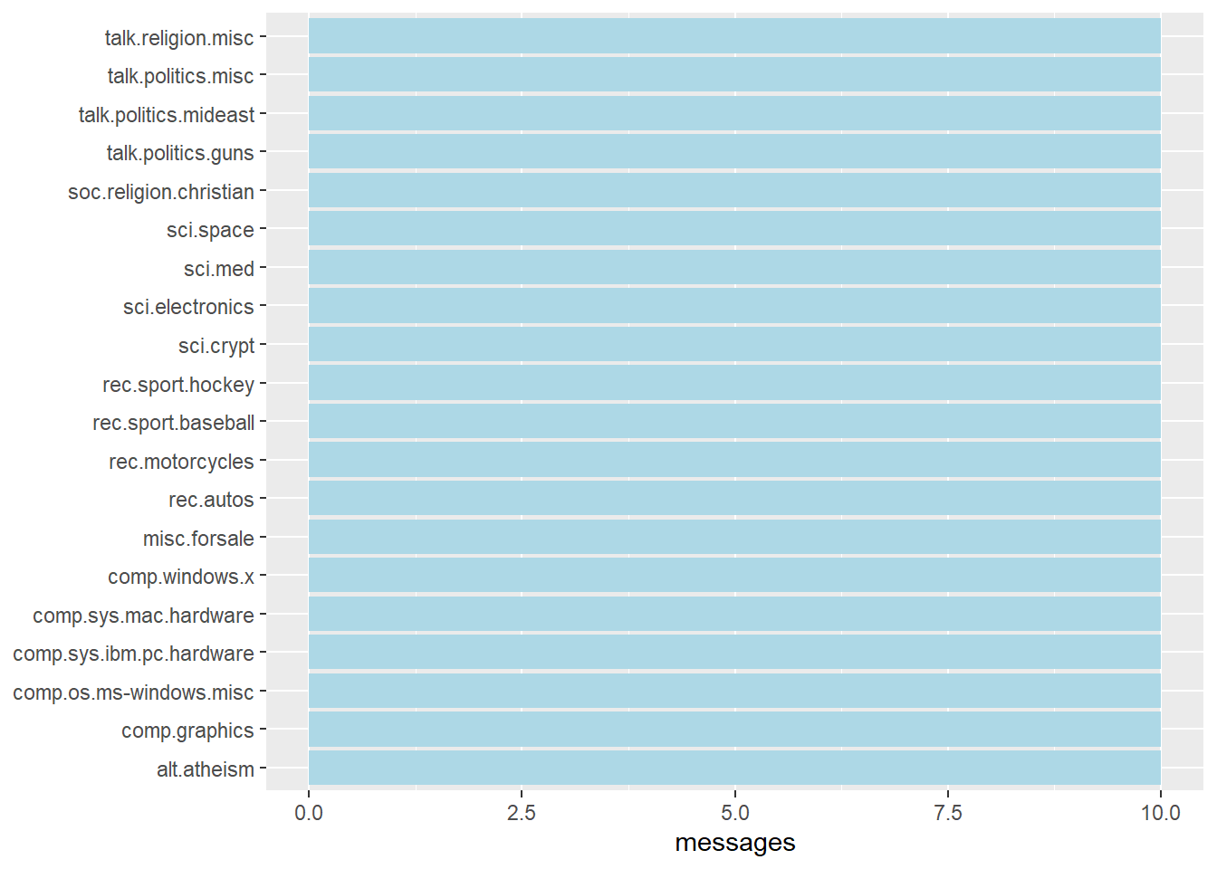
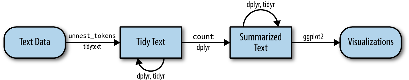
Introducing tidytext
- Using tidy data principles in processing, analysing and visualising text data.
- Much of the infrastructure needed for text mining with tidy data frames already exists in packages like ‘dplyr’, ‘broom’, ‘tidyr’, and ‘ggplot2’.
Figure below shows the workflow using tidytext approach for processing and visualising text data.
Removing header and automated email signitures
Notice that each message has some structure and extra text that we don’t want to include in our analysis. For example, every message has a header, containing field such as “from:” or “in_reply_to:” that describe the message. Some also have automated email signatures, which occur after a line like “–”.
cleaned_text <- raw_text %>%
  group_by(newsgroup, id) %>%
  filter(cumsum(text == "") > 0,
         cumsum(str_detect(
           text, "^--")) == 0) %>%
  ungroup()
Things to learn from the code chunk above:
- cumsum() of base R is used to return a vector whose elements are the cumulative sums of the elements of the argument.
- str_detect() from stringr is used to detect the presence or absence of a pattern in a string.
Removing lines with nested text representing quotes from other users.
In this code chunk below, regular expressions are used to remove with nested text representing quotes from other users.
cleaned_text <- cleaned_text %>%
  filter(str_detect(text, "^[^>]+[A-Za-z\\d]")
         | text == "",
         !str_detect(text,
                     "writes(:|\\.\\.\\.)$"),
         !str_detect(text,
                     "^In article <")
  )
Things to learn from the code chunk above:
- str_detect() from stringr is used to detect the presence or absence of a pattern in a string.
- filter() of dplyr package is used to subset a data frame, retaining all rows that satisfy the specified conditions.
Text Data Processing
In this code chunk below, unnest_tokens() of tidytext package is used to split the dataset into tokens, while stop_words() is used to remove stop-words.
usenet_words <- cleaned_text %>%
  unnest_tokens(word, text) %>%
  filter(str_detect(word, "[a-z']$"),
         !word %in% stop_words$word)
Now that we’ve removed the headers, signatures, and formatting, we can start exploring common words. For starters, we could find the most common words in the entire dataset, or within particular newsgroups.
usenet_words %>%
  count(word, sort = TRUE)
# A tibble: 5,542 × 2
word n
<chr> <int>
1 people 57
2 time 50
3 jesus 47
4 god 44
5 message 40
6 br 27
7 bible 23
8 drive 23
9 homosexual 23
10 read 22
# ℹ 5,532 more rowsInstead of counting individual word, you can also count words within by newsgroup by using the code chunk below.
words_by_newsgroup <- usenet_words %>%
  count(newsgroup, word, sort = TRUE) %>%
  ungroup()
Visualising Words in newsgroups
In this code chunk below, wordcloud() of wordcloud package is used to plot a static wordcloud.
wordcloud(words_by_newsgroup$word,
          words_by_newsgroup$n,
          max.words = 300)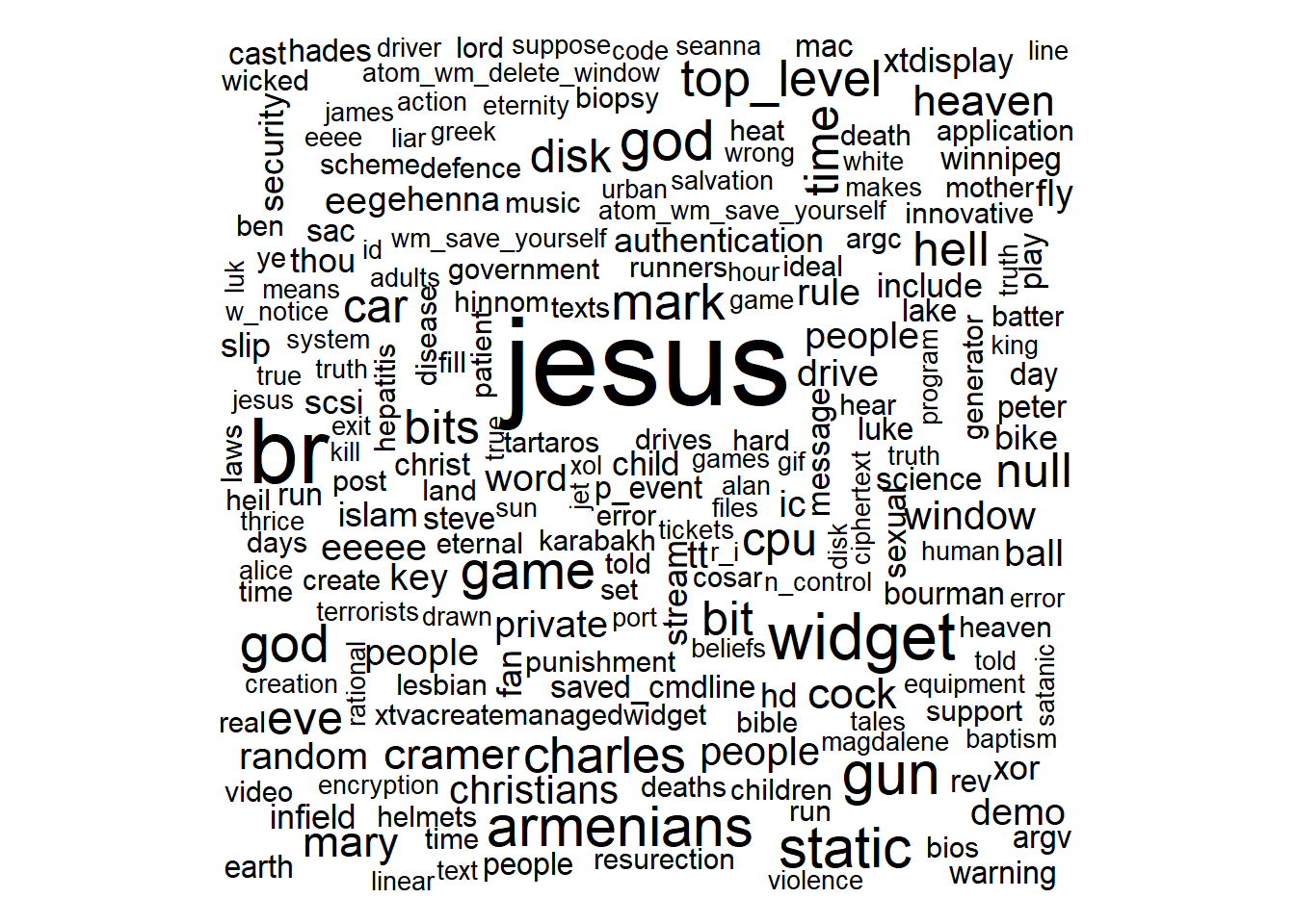
A DT table can be used to complement the visual discovery.
DT::datatable(words_by_newsgroup, filter = 'top') %>%
  formatStyle(0,
              target = 'row',
              lineHeight='25%')
Visualising Words in newsgroups
The wordcloud below is plotted by using ggwordcloud package
set.seed(1234)

words_by_newsgroup %>%
  filter(n > 0) %>%
ggplot(aes(label = word,
           size = n)) +
  geom_text_wordcloud() +
  theme_minimal() +
  facet_wrap(~newsgroup)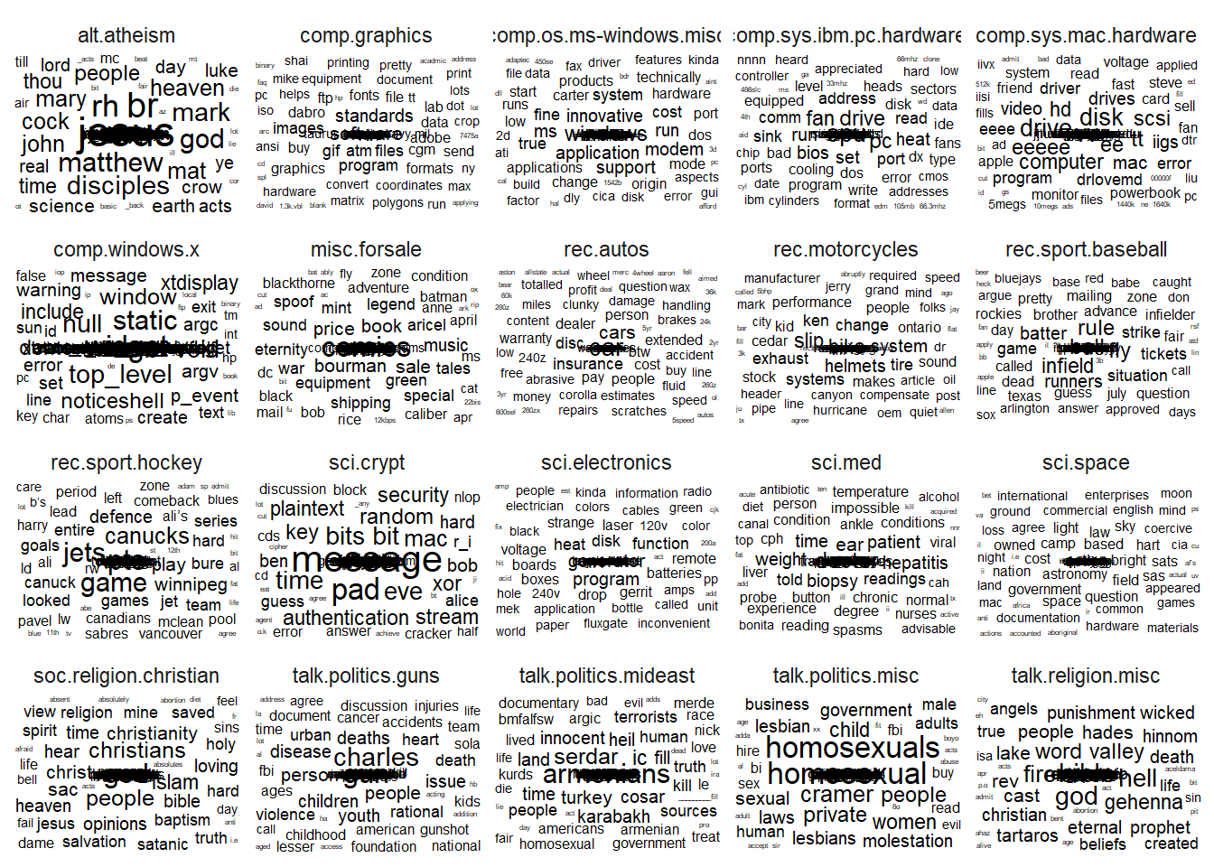
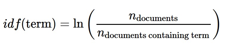
Basic Concept of TF-IDF
- tf–idf, short for term frequency–inverse document frequency, is a numerical statistic that is intended to reflect how important a word is to a document in a collection of corpus.
Computing tf-idf within newsgroups
The code chunk below uses bind_tf_idf() of tidytext to compute and bind the term frequency, inverse document frequency and ti-idf of a tidy text dataset to the dataset.
tf_idf <- words_by_newsgroup %>%
  bind_tf_idf(word, newsgroup, n) %>%
  arrange(desc(tf_idf))
###Visualising tf-idf as interactive table
The code chunk below uses datatable() of DT package to create a html table that allows pagination of rows and columns.
DT::datatable(tf_idf, filter = 'top') %>%
  formatRound(columns = c('tf', 'idf',
                          'tf_idf'),
              digits = 3) %>%
  formatStyle(0,
              target = 'row',
              lineHeight='25%')
Things to learn from the code chunk above:
- filter() argument is used to turn control the filter UI.
- formatRound() is used to customise the values format. The argument digits define the number of decimal places.
- formatStyle() is used to customise the output table. In this example, the arguments target and lineHeight are used to reduce the line height by 25%.
To learn more about customising DT’s table, visit this link.
Visualising tf-idf within newsgroups
Facet bar charts technique is used to visualise the tf-idf values of science related newsgroup.
tf_idf %>%
  filter(str_detect(newsgroup, "^sci\\.")) %>%
  group_by(newsgroup) %>%
  slice_max(tf_idf,
            n = 12) %>%
  ungroup() %>%
  mutate(word = reorder(word,
                        tf_idf)) %>%
  ggplot(aes(tf_idf,
             word,
             fill = newsgroup)) +
  geom_col(show.legend = FALSE) +
  facet_wrap(~ newsgroup,
             scales = "free") +
  labs(x = "tf-idf",
       y = NULL)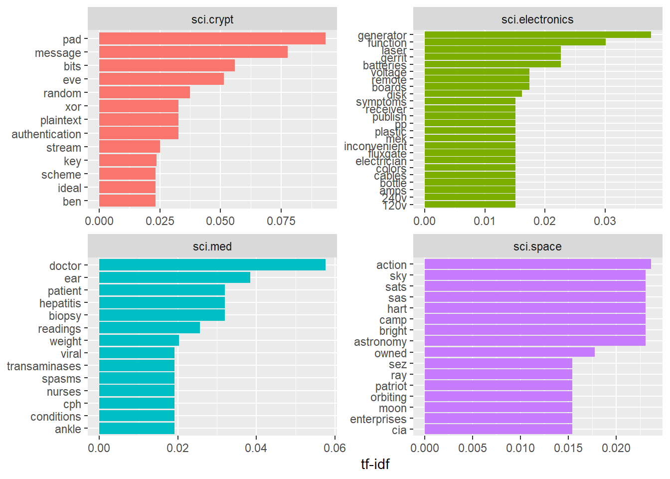
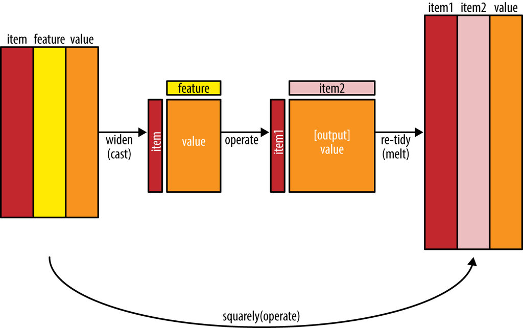
Counting and correlating pairs of words with the widyr package
- To count the number of times that two words appear within the same document, or to see how correlated they are.
- Most operations for finding pairwise counts or correlations need to turn the data into a wide matrix first.
- widyr package first ‘casts’ a tidy dataset into a wide matrix, performs an operation such as a correlation on it, then re-tidies the result.
In this code chunk below, pairwise_cor() of widyr package is used to compute the correlation between newsgroup based on the common words found.
newsgroup_cors <- words_by_newsgroup %>%
  pairwise_cor(newsgroup,
               word,
               n,
               sort = TRUE)
Visualising correlation as a network
Now, we can visualise the relationship between newgroups in network graph as shown below.
set.seed(2017)

newsgroup_cors %>%
  filter(correlation > .025) %>%
  graph_from_data_frame() %>%
  ggraph(layout = "fr") +
  geom_edge_link(aes(alpha = correlation,
                     width = correlation)) +
  geom_node_point(size = 6,
                  color = "lightblue") +
  geom_node_text(aes(label = name),
                 color = "red",
                 repel = TRUE) +
  theme_void()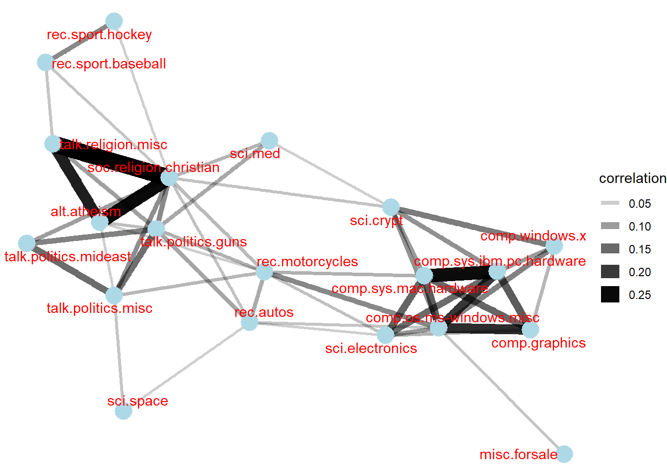
Bigram
In this code chunk below, a bigram data frame is created by using unnest_tokens() of tidytext.
bigrams <- cleaned_text %>%
  unnest_tokens(bigram,
                text,
                token = "ngrams",
                n = 2)
bigrams
# A tibble: 28,824 × 3
newsgroup id bigram
<chr> <chr> <chr>
1 alt.atheism 54256 <NA>
2 alt.atheism 54256 <NA>
3 alt.atheism 54256 as i
4 alt.atheism 54256 i don't
5 alt.atheism 54256 don't know
6 alt.atheism 54256 know this
7 alt.atheism 54256 this book
8 alt.atheism 54256 book i
9 alt.atheism 54256 i will
10 alt.atheism 54256 will use
# ℹ 28,814 more rowsCounting bigrams
The code chunk is used to count and sort the bigram data frame ascendingly.
bigrams_count <- bigrams %>%
  filter(bigram != 'NA') %>%
  count(bigram, sort = TRUE)

bigrams_count
# A tibble: 19,885 × 2
bigram n
<chr> <int>
1 of the 169
2 in the 113
3 to the 74
4 to be 59
5 for the 52
6 i have 48
7 that the 47
8 if you 40
9 on the 39
10 it is 38
# ℹ 19,875 more rowsCleaning bigram
The code chunk below is used to seperate the bigram into two words.
bigrams_separated <- bigrams %>%
  filter(bigram != 'NA') %>%
  separate(bigram, c("word1", "word2"),
           sep = " ")

bigrams_filtered <- bigrams_separated %>%
  filter(!word1 %in% stop_words$word) %>%
  filter(!word2 %in% stop_words$word)

bigrams_filtered
# A tibble: 4,604 × 4
newsgroup id word1 word2
<chr> <chr> <chr> <chr>
1 alt.atheism 54256 defines god
2 alt.atheism 54256 term preclues
3 alt.atheism 54256 science ideas
4 alt.atheism 54256 ideas drawn
5 alt.atheism 54256 supernatural precludes
6 alt.atheism 54256 scientific assertions
7 alt.atheism 54256 religious dogma
8 alt.atheism 54256 religion involves
9 alt.atheism 54256 involves circumventing
10 alt.atheism 54256 gain absolute
# ℹ 4,594 more rowsCounting the bigram again
bigram_counts <- bigrams_filtered %>%
  count(word1, word2, sort = TRUE)
Create a network graph from bigram data frame
In the code chunk below, a network graph is created by using graph_from_data_frame() of igraph package.
bigram_graph <- bigram_counts %>%
  filter(n > 3) %>%
  graph_from_data_frame()
bigram_graph
IGRAPH a48d625 DN-- 40 24 --
+ attr: name (v/c), n (e/n)
+ edges from a48d625 (vertex names):
[1] 1 ->2 1 ->3 static ->void
[4] time ->pad 1 ->4 infield ->fly
[7] mat ->28 vv ->vv 1 ->5
[10] cock ->crow noticeshell->widget 27 ->1993
[13] 3 ->4 child ->molestation cock ->crew
[16] gun ->violence heat ->sink homosexual ->male
[19] homosexual ->women include ->xol mary ->magdalene
[22] read ->write rev ->20 tt ->ee Visualizing a network of bigrams with ggraph
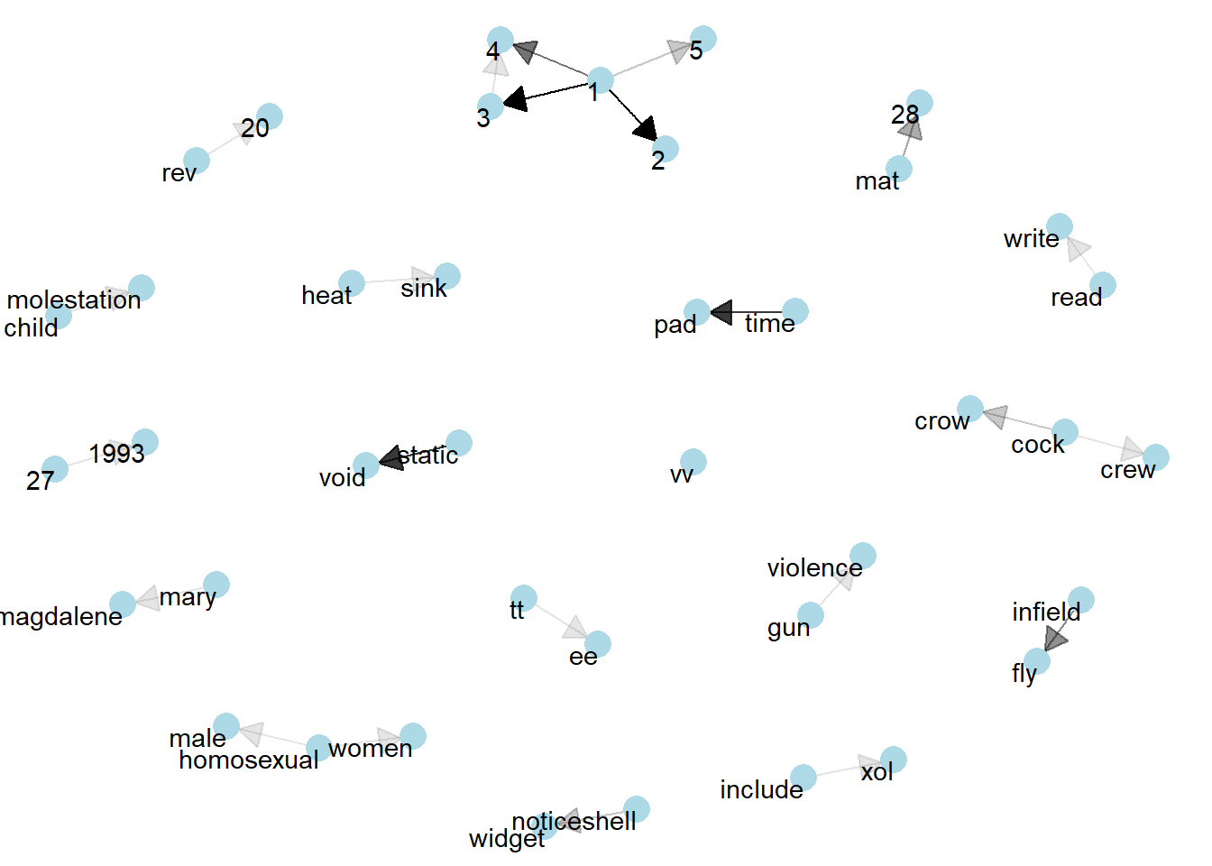
In this code chunk below, ggraph package is used to plot the bigram.
set.seed(1234)

ggraph(bigram_graph, layout = "fr") +
  geom_edge_link() +
  geom_node_point() +
  geom_node_text(aes(label = name),
                 vjust = 1,
                 hjust = 1)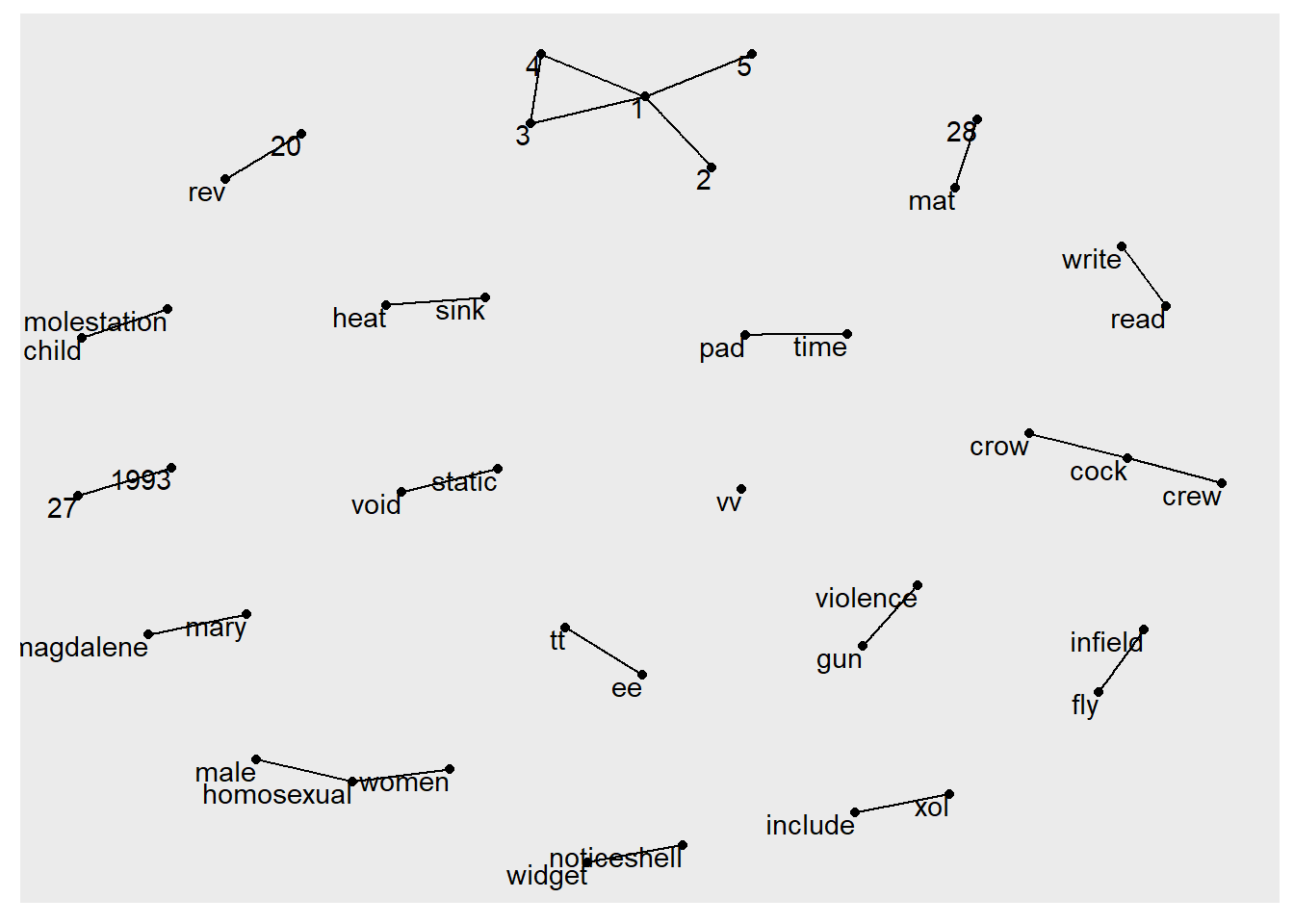
Visualizing a network of bigrams with ggraph
In this code chunk below, ggraph package is used to plot the bigram.
set.seed(1234)

a <- grid::arrow(type = "closed",
                 length = unit(.15,
                               "inches"))

ggraph(bigram_graph,
       layout = "fr") +
  geom_edge_link(aes(edge_alpha = n),
                 show.legend = FALSE,
                 arrow = a,
                 end_cap = circle(.07,
                                  'inches')) +
  geom_node_point(color = "lightblue",
                  size = 5) +
  geom_node_text(aes(label = name),
                 vjust = 1,
                 hjust = 1) +
  theme_void()