In-class Ex6a

Getting started

Installing & loading required libraries

The code chunk below installs and launches the tidyverse, ggdist, ggridges, colourspace & ggthemes packages into R environment

pacman:: p_load(jsonlite, tidyverse, tidygraph, ggraph, visNetwork, graphlayouts, skimr)

Importing the data

The code chunk below imports exam_data.csv into R environment by using read_csv() function of readr package, which is part of the tidyverse package.

The code chunk below imports exam_data.csv into R environment by using read_csv() function of readr package, which is part of the tidyverse package.

mc3_data <- fromJSON("data/mc3_old.json")

class(mc3_data)

[1] "list"

mc3_edges <- as_tibble(mc3_data$links) %>%
  distinct() %>%
  mutate(source = as.character(source), target = as.character(target), type = as.character(type)) %>%
  group_by(source, target, type) %>%
  summarise(weights=n()) %>%
  filter(source!=target) %>%
  ungroup()

mc3_nodes <- as_tibble(mc3_data$nodes) %>%
  mutate(country = as.character(country), id = as.character(id), product_services = as.character(product_services), revenue_omu = as.numeric(as.character(revenue_omu)), type = as.character(type)) %>%
  select(id, country, product_services, revenue_omu, type)

id1 <- mc3_edges %>%
  select(source) %>%
  rename(id = source)
id2 <- mc3_edges %>%
  select(target) %>%
  rename(id = target)
mc3_nodes1 <- rbind(id1, id2) %>%
  distinct() %>%
  left_join(mc3_nodes,
            unmatched = "drop")

mc3_graph <- tbl_graph(nodes = mc3_nodes1,
                       edges = mc3_edges,
                       directed = FALSE) %>%
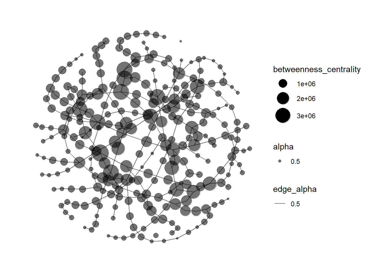
  mutate(betweenness_centrality = centrality_betweenness(), closeness_centrality = centrality_closeness())

mc3_graph %>%
  filter(betweenness_centrality >= 300000) %>%
  ggraph(layout = 'fr') + geom_edge_link(aes(alpha = 0.5)) +
  geom_node_point(aes(
    size = betweenness_centrality,
    colors = "lightblue",
    alpha = 0.5)) +
  scale_size_continuous(range=c(1,10))+
  theme_graph()